

对于数据的敏感,来自对数据的统计,今天我们将基于LDA模型找一篇中文报道找出它的主题,并进行词云绘制
LDA(Latent Dirichlet Allocation)
在 LDA 中,建模过程围绕三件事展开:文本语料库、文档集合、D 和文档中的单词 W。因此,该算法试图通过以下方式从该语料库中发现 K 个主题(如图所示)

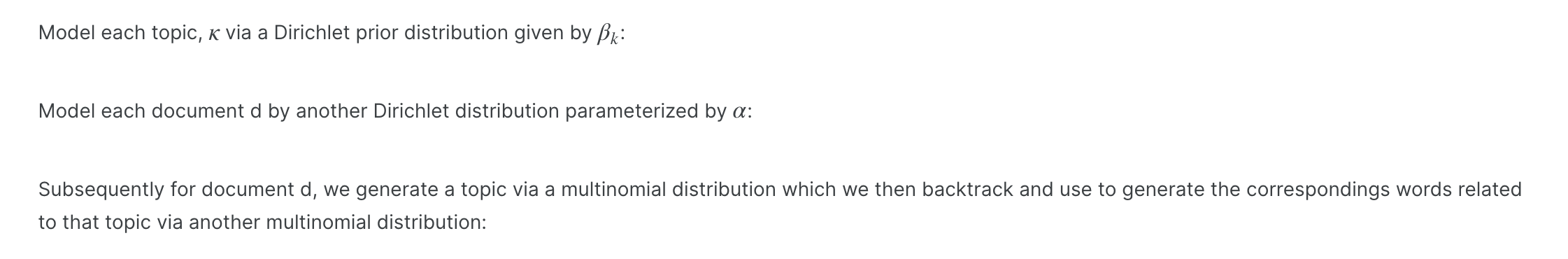 LDA 算法首先通过主题的混合模型对文档进行建模。从这些主题中,然后根据这些主题的概率分布为单词分配权重。正是这种对单词的概率分配允许 LDA 的用户说出特定单词落入主题的可能性。随后,从分配给特定主题的单词集合中,我们才能从词汇的角度深入了解该主题实际上可能代表什么。
数据向量化
我直接复制了今年的一项会议报告,大家最后可以看结果猜一猜是哪个会议
1.首先进行切割成句操作
2.停用词通常是在语料库中出现得如此普遍且频率如此之高的词,以至于它们实际上对学习或预测过程没有多大贡献,因为学习模型无法将其与其他文本区分开来。
3.将文本向量化
import re
import jieba
import nltk
import numpy as np
import pandas as pd
import plotly.io as pio
import plotly.graph_objs as go
from sklearn.decomposition import LatentDirichletAllocation
from sklearn.feature_extraction.text import CountVectorizer
from wordcloud import WordCloud
# 定义中文分词器
def chinese_tokenizer(text):
words = jieba.lcut(text)
return words
def split_sentences_by_punctuation(text):
# 根据标点切割文本
text = text.replace('\n', '')
# 定义一个正则表达式匹配大多数标点符号后面跟着的可能的结束位置
pattern = r'[。!?…;]'
# 使用re.split()函数按照这些标点符号将文本分割成句子
sentences = re.split(pattern + '+', text)
# 去除最后一个元素如果是空字符串的情况
if sentences[-1] == '':
sentences = sentences[:-1]
return sentences
with open('/Users/mac/Desktop/nlp/kaggle/Topic Modelling tutorial/test.txt', 'r') as file:
chinese_text = file.read()
sentences = split_sentences_by_punctuation(chinese_text)
stopwords = nltk.corpus.stopwords.words('chinese')
# 创建CountVectorizer对象,使用自定义的中文分词器
vectorizer = CountVectorizer(tokenizer=chinese_tokenizer,
max_df=0.95,
min_df=2,
stop_words=stopwords,
decode_error='ignore')
# 将文本向量化
tf = vectorizer.fit_transform(sentences)
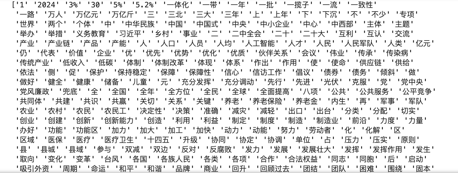
# 打印特征词汇
print(vectorizer.get_feature_names_out())
 数据可视化
数据可视化
plot for the Top 50 word frequencies
feature_names = vectorizer.get_feature_names()
count_vec = np.asarray(tf.sum(axis=0)).ravel()
zipped = list(zip(feature_names, count_vec))
x, y = (list(x) for x in zip(*sorted(zipped, key=lambda x: x[1], reverse=True)))
# Plotting the Plot.ly plot for the Top 50 word frequencies
data = [go.Bar(
x=x[0:50],
y=y[0:50],
marker=dict(colorscale='Jet',
color=y[0:50]
),
text='Word counts'
)]
layout = go.Layout(
title='Top 50 Word frequencies after Preprocessing'
)
fig = go.Figure(data=data, layout=layout)
pio.show(fig, filename='top-50-bar')
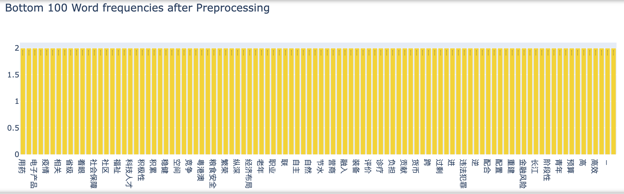
# Plotting the Plot.ly plot for the Bottom 100 word frequencies
data = [go.Bar(
x=x[-100:],
y=y[-100:],
marker=dict(colorscale='Portland',
color=y[-100:]
),
text='Word counts'
)]
layout = go.Layout(
title='Bottom 100 Word frequencies after Preprocessing'
)
fig2 = go.Figure(data=data, layout=layout)
pio.show(fig2, filename='bottom-100-bar')
构建模型
#n_component选了5个主题
lda = LatentDirichletAllocation(n_components=5, max_iter=5,
learning_method='online',
learning_offset=50.,
random_state=0)
lda.fit(tf)
# Define helper function to print top words
def print_top_words(model, feature_names, n_top_words):
for index, topic in enumerate(model.components_):
message = "\nTopic #{}:".format(index)
message += " ".join([feature_names[i] for i in topic.argsort()[:-n_top_words - 1:-1]])
print(message)
print("=" * 70)
feature_names = vectorizer.get_feature_names()
n_top_words = 100
print("\nTopics in LDA model: ")
# 打印每个类别前100个词
print_top_words(lda, feature_names, n_top_words)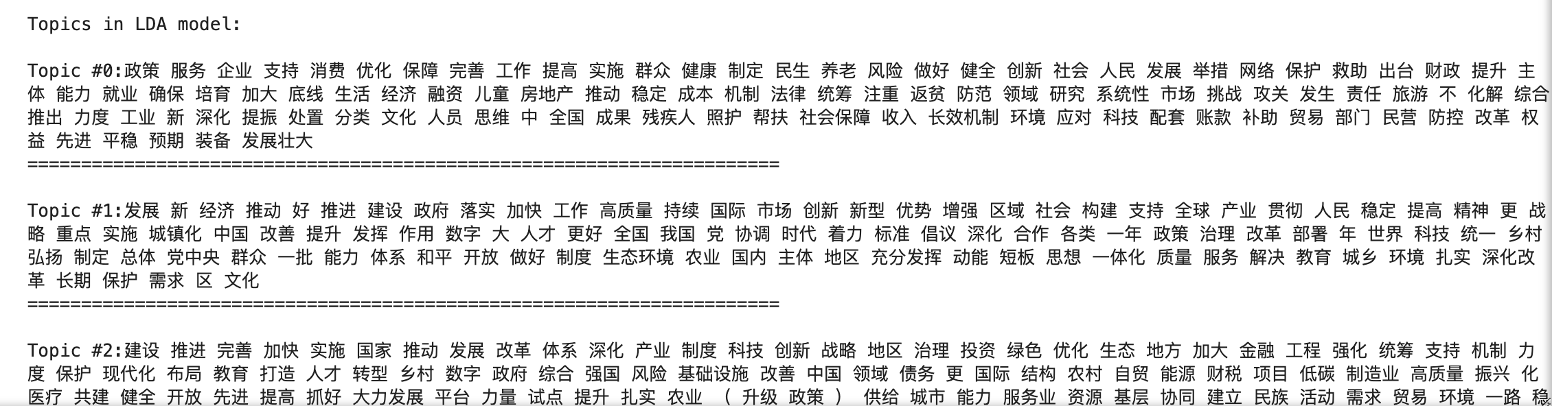 词云绘制
词云绘制
from wordcloud import WordCloud, STOPWORDS
import matplotlib.pyplot as plt
# 我这里只取了第一类数据前80个词
first_topic = lda.components_[0]
# second_topic = lda.components_[1]
# third_topic = lda.components_[2]
# fourth_topic = lda.components_[3]
first_topic_words = [tf_feature_names[i] for i in first_topic.argsort()[:-80 - 1 :-1]]

firstcloud = WordCloud(font_path="/Users/mac/Library/Fonts/MaShanZheng-Regular.ttf",
                       width=800, height=600, mode='RGBA')
firstcloud.generate(" ".join(first_topic_words))
plt.imshow(firstcloud)
plt.axis('off')
plt.show()
文章参考:
文章参考: